

Logistic Regression from scratch (and how to make it nonlinear)
Logistic Regression is a staple of the data science workflow. It constructs a linear decision boundary and outputs a probability. Below, I show how to implement Logistic Regression with Stochastic Gradient Descent (SGD) in a few dozen lines of Python code, using NumPy. Then I will show how to build a nonlinear decision boundary with Logistic Regression by using feature crosses.
Here is the repo with the full code shown below.
Why logistic regression?
Although, in many applications Logistic Regression has been replaced by more advanced techniques such as ensemble tree-based methods (like gradient boosting) or by deep neural networks. However, it is still commonly used due to its simplicity and interpretability. For example, the algorithm is still a workhorse in some applications such as credit risk where legal considerations highly value its simplicity.
In addition, Logistic Regression is still important for many reasons including: it serves as a simple-to-train baseline, works well with sparse features, adds memorization capabilities, as in a wide and deep model, and is simple and easy to implement.
Finally it serves as a nice learning aid for deep learning, as logistic regression is equivalent to a neural network with no hidden layers. Like neural networks, you can train it using stochastic gradient descent.
Always start with a baseline
Baselines are important. Before you start building complex models, test your features on a simple model – this will save you valuable debugging time and help you figure out if there is indeed signal in your data. The time to train Logistic Regression models (and ensemble methods such as Random Forest) is typically at least an order of magnitude faster than that of deep neural networks.
It’s cheap to realize your data is crap or to debug data leakage on your simple model that takes seconds to train, rather than your complex one that takes minutes to hours.
Finally, a baseline model gives you an initial target to beat. If you can’t beat your baseline with a complex model or you are just barely beating it, stick to your baseline or go back to the drawing board.
Logistic Regression in NumPy
Here is the entire code to train Logistic Regression from scratch in Python.
BATCH_SIZE = 100
STEPS = 1000
LEARNING_RATE = 0.5

def _sigmoid(logits):
    return 1/(1 + np.exp(-logits))

def forward(X, W):
    logits = np.dot(X, W)
    return _sigmoid(logits)[:,0]

def gradient(X, y, pred):
    return np.dot((pred - y), X).T/y.shape[0]

def get_next_batch():
    return df.iloc[start:end,:][features], df.iloc[start:end]['y']

# initialize
start = 0
end = BATCH_SIZE
W = np.random.random([N_FEATURES, 1])

for step in STEPS:

    X_batch, y_batch = get_next_batch(traindf)
    pred = forward(X_batch, W)
    dw = gradient(X_batch, y_batch, pred).reshape(N_FEATURES,1)
    W -= LEARNING_RATE*dw

    start += BATCH_SIZE
    end += BATCH_SIZE
    LEARNING_RATE *= .99
Let’s walk through the key parts of the code. The forward call creates predictions by multiplying the model’s weights by our input vector containing our features (the input includes the bias value) and summing the result.
def _sigmoid(logits):
    return 1/(1 + np.exp(-logits))

def forward(X, W):
    logits = np.dot(X, W)
    return _sigmoid(logits)[:,0]
In order to actually train the model, we need to iteratively update the weights at each step using the gradient approximation from each batch. The lecture notes from Andrew Ng’s cs229 course provide a nice derivation of the weight update step.
def gradient(X, y, pred):
    return np.dot((pred - y), X).T/y.shape[0]
In our case, we will be using vanilla Stochastic Gradient Descent (SGD) for training out model. SGD is the workhorse for training our model. Alternatively, we could utilize more sophisticated optimizers such as Adam or Momentum Optimizers, which would likely converge faster. Below if the iterative updating process for SGD.
for step in STEPS:
    X_batch, y_batch = get_next_batch(traindf)
    pred = forward(X_batch, W)
    dw = gradient(X_batch, y_batch, pred).reshape(N_FEATURES,1)
    W -= LEARNING_RATE*dw. # SGD update step
Let’s try our algorithm on a dataset consisting of two features and a linear separating boundary. It successfully learns a boundry to do so:
Our model will run into difficulty trying to classify examples created from the XOR function. There is no single line that can differentiate the two classes.
Feature crosses introduce nonlinearity
Edit: Regarding the term nonlinear. As some readers have pointed out, Logistic Regression is not linear as defined by the definition of linearity: when an input variable is changed, the change in the output is proportional to the change in the input. See the sigmoid function, which is clearly nonlinear. See this post for more info.
However, Linear Regression is a linear classifier (which is what I’m referring to) as the prediction is based on the value of a linear combination of the inputs. By adding feature crosses you change this and thus are not restricted to a hyperplane decision boundary. Also if you are confused by term feature crosses… feature cross = interaction variable.
We can incorporate feature crosses to solve the XOR problem. This will give the classifier more to work with than just a “line” to seperate classes. Feature crosses allow us to build nonlinear decision boundaries, even though we are using a linear classifier, logistic regression.
This is important because many real world phenomena are nonlinear. I’ll show an intuitive example of feature crosses below on the titanic dataset.
We can cross f1 and f2 by multiplying them together:
df['f1f2'] = df['f1'] * df['f2']
Let’s revisit the XOR problem using feature crosses:
Using additional crosses, we can solve even more shapes.
A distribution created from a sinewave function:
The model can’t quite fit a box, but it’s better than without crosses, using just a line.
Just be careful of overfitting. Feature crosses, particularly for categorical variables, blow up the feature space and can be cause your model to overfit. Incorporating regularization becomes even more important.
While this example is nice to view visually, let’s look at feature crosses on the Titanic dataset.
Feature crosses: Intuitive example using titanic
The titanic dataset is a rather morbid dataset, for predicting if a passenger will survive or die on the titanic cruiseliner. There are several features available, but I will just be using a couple:
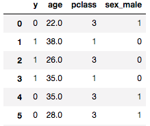
Using the logistic regression code I wrote above, I ran 100 trials:
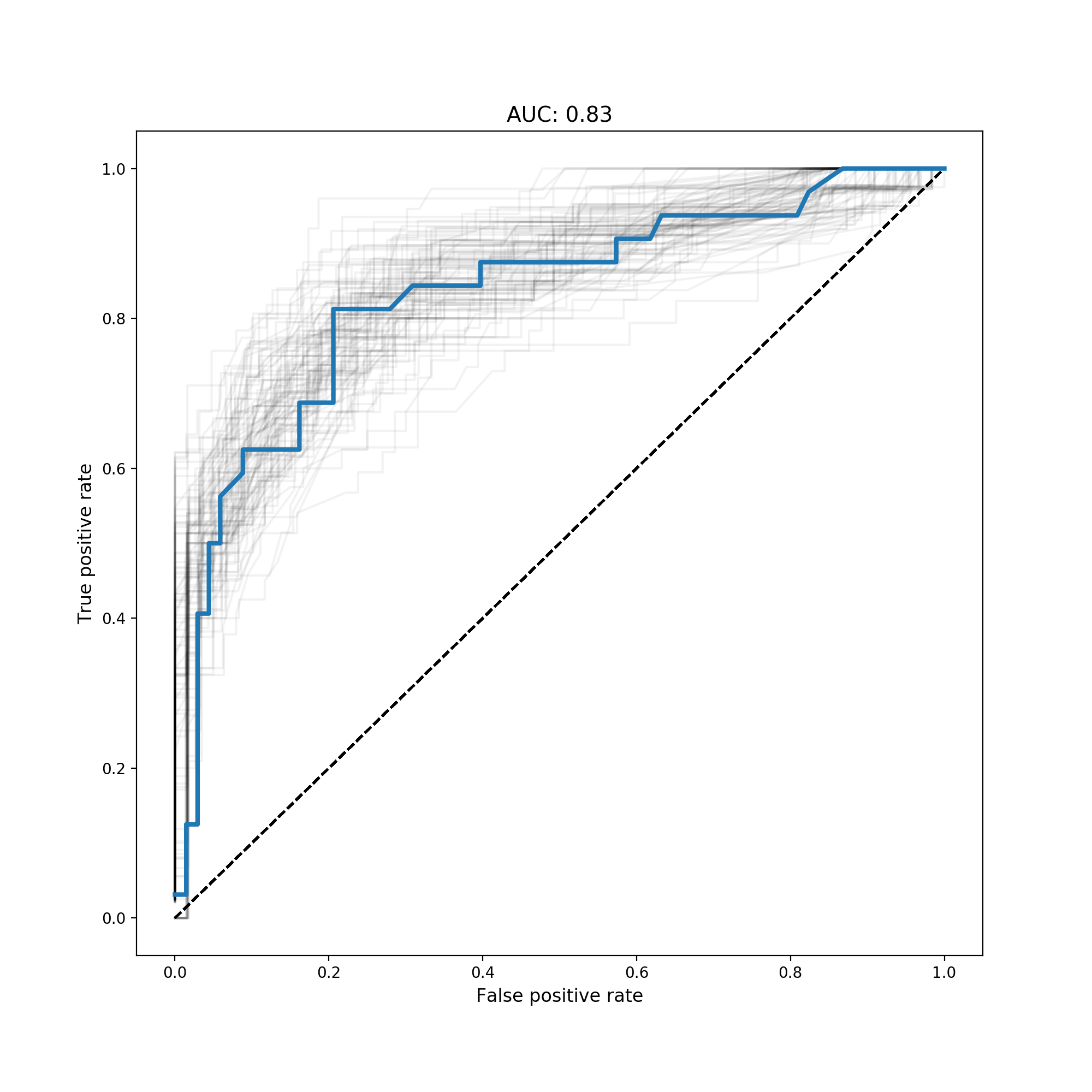
Let’s cross sex_male with age. The hypothesis being that both age and gender, together, affected one’s likelihood to survive. We know gender and age by themselves are important - there is the line “women and children first” that was alledged to be said for who has access to life rafts. Thus age and sex_male are both negatively correlated with survival.
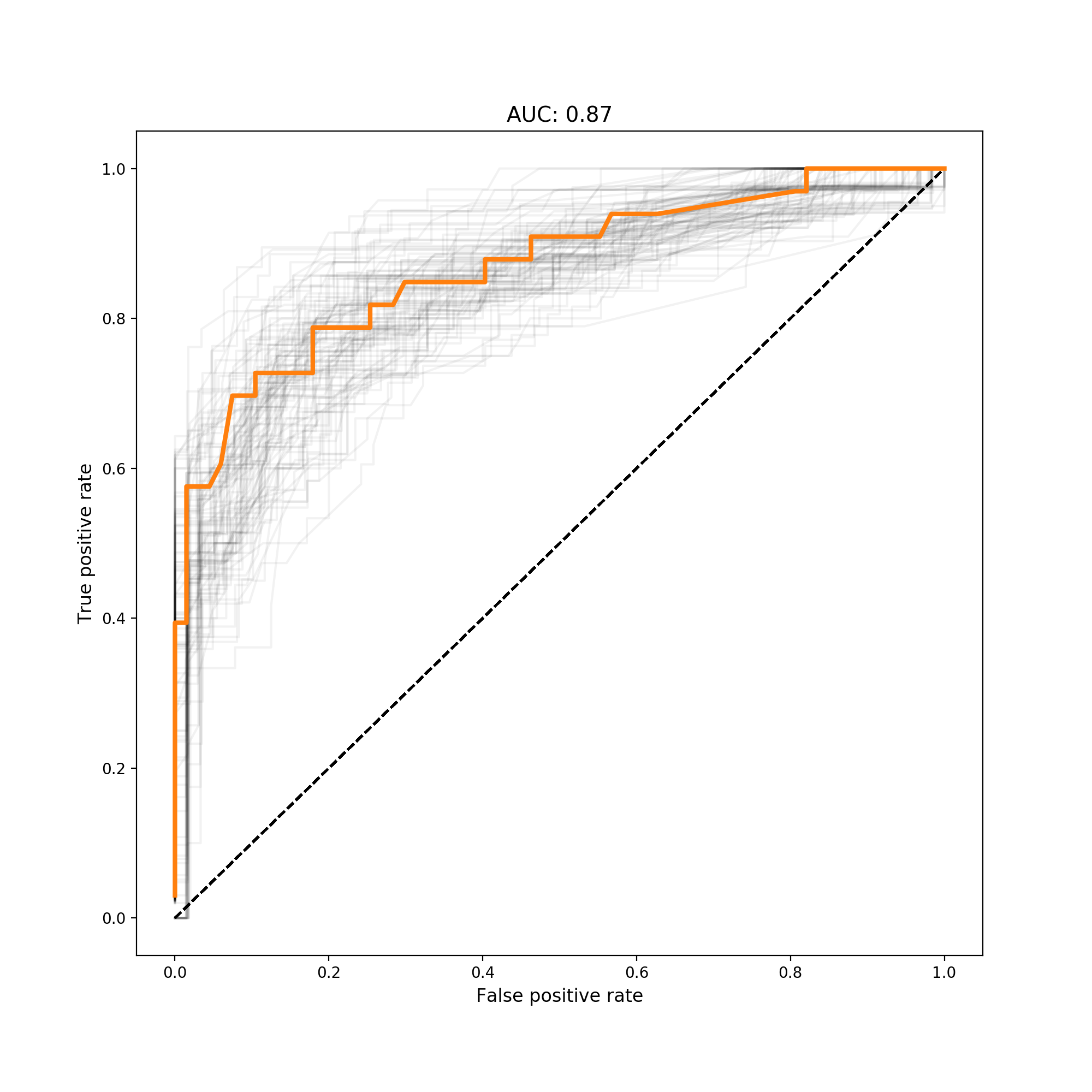
However, what about gender for children? It wasn’t the case that girls were more likely to survive then boys. Right now the model doesn’t encode this relationship. We need to cross the two features to create age__x__sex_male:
After crossing these two columns, we get better AUC:
Conclusion
Logistic regression is relatively simple to implement from scratch. Though it’s been around for decades, it still is heavily utilized and serves as a nice instructional tool for learning more advanced techniques like neural networks. Finally, though it’s a linear classifier, logistic regression can create nonlinear decision boundaries if input features are crossed.
Additional Resources
- Feature Crosses in TensorFlow, Scikit-Learn
- Try feature crosses (and training deep neural networks) interactively with TensorFlow playground.
- Quora answer on linearity and logistic regression


